Publish to Excel Services
The first version of our workbook is now complete and ready to be published to our SharePoint site:
In
Excel, click the File menu to enter the backstage area. Select Share
from the list of options and then select Publish to Excel Services.
Set the path to http://localhost/Example/Excel Workbooks and the filename to Last30DaysSales.xlsx.
Click to save the file to SharePoint.
Tip
When using Excel 2010 on
Windows 2008 server, trying to save files to SharePoint doesn’t quite
work as it should. This is because the WebClient service that maps the
SharePoint URL to a UNC path behind the scenes, isn’t configured by
default since it has no purpose on a server operating system. To fix
this problem, install the Desktop Experience feature using Server
Manager.
Create a User Interface Using the Excel Web Access Web Part
Now that we have our workbook
published to SharePoint, we can move on to make use of it when
generating a user interface for our sample application. We’ll customize
the homepage of our site to include our sales chart.
Navigate to http://localhost/Example/Default.aspx. From the Site Actions menu, choose Edit Page.
In the Left Web part zone, click Add A Web Part.
Select
the Excel Web Access (EWA) web part from the Office Client Applications
category. Click Add to include the web part on the page.
Note
If this web part is missing
from the web part gallery, ensure that the SharePoint Server Enterprise
Site Features and SharePoint Server Enterprise Site Collection Features
are enabled for the current site and site collection.
To set the properties of the web part, click the Click Here To Open The Tool Pane link.
In the Workbook Display section, type the workbook as /Example/Excel Workbooks/Last30DaysSales.xlsx.
Since we’re interested only in the chart for now, in the Named Item field type Chart 1. Click Apply to see the results.
We’ve now got our PivotChart
on the page ready for use. Let’s tidy up a few of the remaining web part
settings to give the page a more integrated look:
Set the Type of Toolbar to None. This will hide the toolbar that appears above the chart.
In the Appearance section, set the Chrome type to None.
Click OK to commit the changes and stop editing the web part.
From the Page ribbon, click the Stop Editing button to switch back to View mode.
Adding Interactivity Using a Slicer
New in 2010—You’ve
seen how easy it is to make use of Excel data on a page when using the
Excel Web Access web part. Let’s move on to look at an example of the
interactive features available via the web part. Our demonstration
scenario requires that the data displayed in our chart be filterable
using geographical locations. Although we have listed multiple series,
one for each country code, at the moment we don’t have any way to select
which series should be displayed on the chart.
This section
introduces the Slicer, one of the new features available in Excel 2010
that works very well with Excel Services. Before we can use a Slicer, we
need to add it to our Excel workbook.
Navigate
to the Excel Workbooks document library at http://localhost/Example.
Open the Last30DaysSales.xlsx file using Microsoft Excel by
right-clicking the file and selecting Edit in Microsoft Excel from the
context menu.
Note
that the workbook opens in Protected View mode. This happens because
the workbook is opened from a web site as opposed to a local folder.
Click Enable Editing to proceed.
The
next warning we receive says that “Data Connections have been
disabled.” This is a standard security feature of Excel that prevents
active content from running until it is explicitly allowed. Click Enable
Content to refresh the connected data.
We
have the option to make the document trusted. Click Yes, and the
workbook won’t open in Protected View mode each time. This is OK since
we’ll be doing a bit of work with it.
Adding a Slicer is simple. Select the PivotChart and then, from the Analyze menu, click the Insert Slicer button.
From the Insert Slicers dialog, check the Territory checkbox and then click OK to add the Slicer to our worksheet.
To see the Slicer in action, try selecting one or more (by holding down the CTRL
key while clicking) of the listed Territory values. We can see that the
PivotTable data is filtered based on our selection and the PivotChart
is redrawn accordingly.
Grouping Excel Items for Display Purposes
Since we want to display
only the Slicer and chart on our web page, we need to lay them out in a
specific manner. We now need to display the chart and the Slicer, and
since we can enter only one named item, we need to group these into a
single item.
As you’ve seen earlier,
named ranges can be defined by selecting a range of cells and then
adding a name. We’ll use a named range to refer to our chart and Slicer
control.
Place the chart and the Slicer next to each other on the sheet.
Resize
the chart and the Slicer so that they fill entire cells as much as
possible. This will reduce unnecessary white space when the control is
rendered in the web page. The zoom function is very useful for this
purpose.
Select the underlying range using one of the methods described earlier and type the name ChartAndSlicer in the Name box.
Click
the Save icon in the upper-left corner to save the changes to
SharePoint. We’ll keep the workbook open for now since we’ll be making
additional changes later.
If we now open the home page of
our sample site using Internet Explorer, unsurprisingly we’ll find that
our chart is still there just as before, without our new Slicer control.
One thing that may be apparent is that the chart now shows only the
territories that we selected earlier when we were messing around with
the Slicer in Excel client. Note that slicer selections are published
along with the workbook, so it’s important to make sure that an
appropriate default is set before saving.
Let’s move on to change our Excel Web Access web part to display our Slicer as well as our chart.
From the SiteActions menu, select Edit Page.
Highlight
the Excel Web Access web part by clicking the header; then, from the
Web Part Tools tab, select Web Part Properties from the Options menu.
Change the Named Item to ChartAndSlicer. Click Apply to view the change.
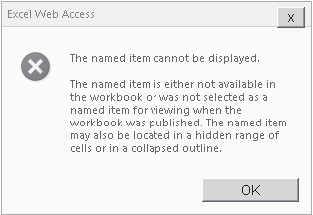
Our
recently defined named item should be displayed on the page, but,
instead, we’re presented with the following error message stating that
the named item cannot be displayed:
Click
OK to acknowledge the error message. Then from the Page menu, select
Stop Editing. The page will now be blank except for the error message.
Change Published Items Within a Workbook
When
we initially published our workbook to Excel Services, we simply gave
it a name and accepted the default values. Whenever we click the Save
icon, rather than re-publishing the workbook, we’re merely saving the
data back to the document library. The significance here is that when
publishing a workbook to Excel Services, we have the option of
specifying additional metadata, but when saving, the metadata is not
changed. We received the error because the metadata did not contain
details of our new named item.
Switch back to Excel client. Click the File menu to enter the backstage area. Select the Share option, as shown:
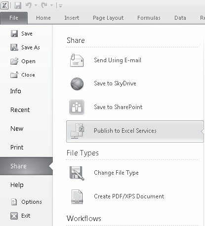
The
Share section offers two options: Save to SharePoint and Publish to
Excel Services. As described, the difference between these two options
is the ability to add metadata that’s useful to Excel Services. Let’s
see what that means in practice. Click Save to SharePoint.
Click
the Current Location icon to open the Save As dialog, which
automatically displays the contents of our Excel Workbooks document
library and allows us to save the workbook in the normal manner. Click
Cancel and then return to the Share section of the backstage area.
This
time, click Publish To Excel Services to open the Save As dialog, but
notice that an Excel Services Options button now appears in the bottom
section of the dialog.
Click
the Excel Service Options button to define or overwrite metadata for
the document. In the Excel Services Options dialog’s Show tab, select
Items In The Workbook from the drop-down list.
Check the All Named Ranges and the All Charts options to ensure that they will be available for use by the EWA web part.
Note
At the time of writing, a bug (or
feature, depending on your point of view) exists within Excel 2010.
Named ranges that are blank are not detected by the Excel Services
publishing process and therefore don’t appear in the list of Items in
the workbook. To resolve this issue, select the ChartAndSlicer named
range and press the SPACEBAR. This will ensure that the range appears in the list of metadata.
Click Save to complete the publishing process.
With our metadata updated
appropriately, if we return to the sample site home page, we can see
that our EWA web part now displays our chart and Slicer as expected. The
Slicer behaves in much the same manner as we saw earlier when we used
it within the Excel client application.